


ISSN: 0973-7510
E-ISSN: 2581-690X
Existing culture-based instruments for detecting/quantifying proliferating bacteria in suspensions (BACTECTM, BacT/AlertTM, RABITTM etc.) do so based on changes observed in the physical/chemical properties of media (O2/CO2 levels, pH etc.) due to bacterial metabolism. Given the limited metabolic-rate of individual bacterium, they have a “threshold-concentration” of ~107-108CFU/ml, and Times to Detection (TTDs) of 12 hours or longer for low initial loads (<100CFU/ml). We recently developed a method that tracks microbial proliferation in suspensions by monitoring the degree of cell polarization of live microorganisms. In the presence of an AC electric field, there occurs a build-up of charge at the microbial membrane, causing them to act like capacitors. As microorganisms multiply, there occurs a corresponding increase in charges stored in the suspension (“bulk-capacitance”), and this increase in bulk-capacitance serves as our “signature” for presence of live microorganisms. In this study, we explain the theory underlying our approach, establish its applicability to a variety of microorganisms, showing that the “Threshold-Concentration” (nT) for detection is ~103-104CFU/ml, and TTDs are a function of the initial-load(n0) and doubling-time(tD) of the microorganism TTD=1.443*tD*ln(nT/n0) and show that the method can be adapted to obtain the “Most Probable Number” (MPN) of coliforms within 6hrs (vs. >24hrs for existing methods).
Viable bacteria; MPN; Rapid Detection; Automated Culture Systems; Bacteria detection; Microfluidics.
Despite recent advances in detection technologies that make it possible to detect, identify and/or quantify pathogens present in clinical, food, environmental and other samples (such as PNA-FISH®, GeneXpert®, BioMark™, BiacoreTM, SensiQTM, etc) there remains a class of “real world” situations where these technologies do not work. In these situations, one seeks to determine whether there are any viable and proliferating micro-organisms present in a sample with the understanding that, even if present, their concentrations will be very low (100 Colony Forming Units (CFU)/ml or lower), and that it is very likely that the sample will also contain a larger number of dead micro-organisms.
In some cases, such as in assaying process water used for manufacturing pharmaceuticals1, one needs to conduct tests to verify that, after the sterilization processes adopted, there are absolutely no live microorganisms remaining in the entire batch. The goal of such tests is to detect any surviving micro-organism(s), if present.
In other cases, the number of live microorganisms remaining must also be quantified. For instance, the US Department of Agriculture (USDA) requires that ground beef contain <1 CFU of viable E coli per 25g of beef. Even after sample processing to kill bacteria, one still needs to provide proof that the levels of viable bacteria are at or below the approved limits. Using current technologies, it is often the case that by the time the counts of viable bacteria become available (2+ days), the product has often already been shipped. If the counts exceeded the approved limits, the product must be recalled. Every year (since 1997), an average of about 4,500 Metric Tons of meat and poultry are recalled by US industries2. Another instance in which rapid quantification is desired is in the handling and distribution of milk. The US Pasteurized Milk Ordinance3 requires “Grade A” pasteurized milk to have a total viable bacterial count of d” 20,000 CFU/ml and a (viable) coliform count of d” 10 CFU/ml. The USDA Economic Research Service estimates that about 19 million lbs of milk are spoilt each year4. Although, it is theoretically possible to prevent spoilage by re-sterilizing / re-pasteurizing the milk after the bacterial spores that survived sterilization have germinated into vegetative bacteria, by the time current on-line sensors like “electronic noses” (gas sensors / chromatographs), FTIR sensors etc are able to detect a change in the composition of the milk brought about by bacterial metabolism, it is often too far spoilt to be useful (humans will feel changes in taste etc.) and must be discarded, or diverted to other use4.
Also, the Environmental Protection Agency (EPA) specifies that concentration of viable coliform bacteria should not exceed 500 CFU / 100ml for primary contact recreational waters (lakes and beaches) and 800 CFU / 100ml for secondary contact recreational waters (streams)5. Existing technologies for measuring the levels of coliform bacteria have a turnaround time of greater than 1 day (usually 2-3 days). Thus, a particular beach or resort will not be immediately aware of increased risks to users. On the other hand, after the risk has been identified (and actions such as chlorination undertaken), it takes a similarly long time to ascertain that the bacterial counts are back to acceptable levels. The former leads to spread of disease among users, and the latter leads to economic losses. In 2008, the number of closing and advisory days at ocean, bay and Great Lakes beaches topped 20,000 for the 4th consecutive year6. The EPA has, consequently, also announced that it will prioritize the approval of technologies that can quantify the loads of proliferating coliforms in recreational waters in < 1 day.
In these, and related situations, the technologies used continue to be “culture”-based. Here, to detect the presence of proliferating microorganisms, samples are added to a known volume of sterile microbial growth media. If present, proliferating microorganisms metabolize, consuming glucose and oxygen, and releasing lactic/pyruvic acid, CO2 etc. The metabolic activity thus leads to changes in the properties of the surrounding medium such as a decrease in pH, an increase in conductivity, or a change in levels of O2 or CO2. If such changes are detected, they can be taken to indicate the presence of proliferating microorganisms in the sample added to the growth media. This approach forms the basis of a large number of commercial products such as the BACTECTM and BacT/AlertTM that detect changes in CO2 levels7-8, the Difco-ESP SystemTM that monitors pressure changes due to gas consumption or production9, and the BactometerTM and RABITTM that monitor the conductivity of the growth medium10-11. These instruments work very well for wide variety of applications because the presence of dead microorganisms does not affect the results, and that the theoretical Limit of Detection (LOD) is 1 CFU. They are also conducive to automation, keeping the costs low, and thus leading to their popularity.
These instruments, however, suffer from one major drawback: the time taken to detect the presence of living microorganisms is considerable (hours to days)12, especially when initial loads present are low (< ~100 CFU/ml). This is because the detection can be done only when the cumulative effect of microbial metabolism (and proliferation) changes the quantity that they monitor (O2/CO2 levels, pH, conductivity etc.) by a measureable degree. But the rate of metabolism of individual cells is inherently limited. For instance, even a relatively fast growing/metabolizing bacterium like E coli consumes only 2 x 10-14 moles of O2 per hour13, whereas a typical well-oxygenated suspension has a dissolved O2 concentration14 of ~ 10-6 moles/ml. Hence, with the current systems, one has to wait for the concentration of living microorganisms to reach a “threshold” of ~106 to 108 CFU/ml before their metabolism can change the medium properties (O2/CO2 concentration, pH, conductivity etc) to a measurable degree15. The time that elapses before a change in the medium properties is measured (and the presence of live microorganisms in the original culture inferred), is referred to as the Time to Detection (TTD). The TTD typically depends on the initial load of proliferating microorganisms in the sample and the metabolic rate of these microorganisms. In general, TTDs are longer for samples with lower initial loads and for microbes with slower metabolic rates (longer doubling times). The extremely limited amount of metabolites generated/consumed also limits how much TTDs can be reduced by improving the performance of sensors to detect changes in pH, O2/CO2 levels etc. One approach to reducing TTDs that has had some success is the pre-concentration of cells/particles prior to culture, using methods such as filtration16, centrifugation16, immunomagnetic separation17 or dielectrophoresis (DEP)18. But not only do these processes themselves take time and require additional resources, their efficiency of capture is often not 100%, leading to potential false negatives and/or errors in establishing the count. Moreover, since after pre-concentration, the samples are assayed using the same “slow” culture based methods, the benefits of using pre-concentration is also rather limited.
Hence, there is clearly a need for a technology that can reliably detect small numbers of proliferating bacteria in suspensions containing large numbers of dead bacteria (and also other non-living species) in as short a time as possible, and in some cases, accurately quantify the numbers present. It would perhaps also be preferred (given the inherent limitations discussed above) that this method did not rely on detecting the effects of microbial metabolism. In this work, we describe in detail a method that meets both these criteria.
Briefly, our method relies on the microbial polarizability in the presence of high frequency AC electric field there occurs a buildup of charge at the cell-membrane of proliferating cells, causing these cells to behave like electrical capacitors. The proliferation of any viable microorganism present (an increase in the number of live microbial cells) increases the “bulk capacitance” of the sample under investigation, and this increase in bulk capacitance serves as our “signature” indicating the presence of live microorganisms. Confining the sample to a long narrow channel increases the resistance of the solution, and this amplifies the influence of microbial charge storage on the measured impedance (by increasing the effective RC-time constnat). A variant of impedance spectroscopy is used to estimate the charge storage with high sensitivity, and are able to detect microbial proliferation. In our previous work, we reported using this approach to detect E coli in substrates such as food matrices (milk and apple juice)19 and Blood Culture broths20. In both cases, our “threshold concentrations” (at which we were able to infer the presence of living microorganisms) was ~ 103-104 CFU/ml (compared to 106-108 for current systems), and hence our TTDs were 4-10 times smaller than those obtained using current systems.
In this work, our aim is to (a) explain the theory underlying our approach (b) establish that this method is applicable to a variety of proliferating microorganisms (aerobic bacteria, anaerobic bacteria, yeasts, and molds), and that the threshold concentrations are similar for different microorganisms (c) investigate how the Time to Detection (TTD) varies as a function of the initial load (n0) and doubling time (tD) of the microorganism; and (d) show that the method can also be adapted to obtain the “Most Probable Number” (MPN) of proliferating bacteria of interest.
Theory and calculations
Basic principle
It has previously been known21 that, in the presence of high frequency AC electric fields (fields that rapidly change polarity), there occurs a buildup of charge at the cell-membrane of viable cells because these charge carriers (ions) are unable to penetrate through the membrane. Thus, these cells behave like electrical capacitors. Notably, this effect (membrane polarization in an AC field) is lost when the membranes lose their integrity and/or become permeable to charge, such as on cell death22-23. Thus living cells contribute to the “Bulk Capacitance” of a suspension (a measure of the charge that is stored in its interior).
In theory, any increase in number of viable cells (due to proliferation) should result in an increase in the Bulk Capacitance of a suspension. But the Bulk Capacitance is not readily measurable. The cause of the difficulty can be appreciated by studying the electrical representation of an aqueous suspension, as shown in Figure 1(a)24-25. Different components in the circuit shown in Figure 1(a) arise due to the different effects of the applied electric field on the solution/suspension. The flow of ions through the solution (and the viscous resistance to the same) is accounted for by the bulk resistance (Rb); the interfacial resistance (Re) and inductance (Le) are those of the electrodes themselves and that of the wires connecting them to the impedance analyzer; the electrochemical “double layers” formed on the surfaces of charged metal electrodes are accounted for by the Interfacial Capacitance (Ce); and the charges stored in the interior of the suspension are accounted for by the Bulk Capacitance (Cb). The interfacial capacitance is typically ~ 10-8– 10-9 Farads, whereas bulk capacitances are typically ~ 10-12 Farads26. Thus, the interfacial capacitances usually “screen” the bulk capacitance, making it difficult to observe small changes in the latter.
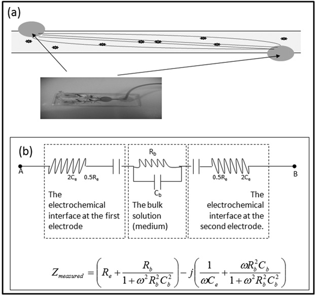
Fig. 1: Microfluidic channel and the corresponding equivalent circuit (a) Schematic representation of the micro-channel with electrodes on either end loaded with suspension with bacteria (The actual image shown in the inset). The spatial confinement of the electrical lines of force ensure sensitivity of electrical measurements to the bacteria present (b) Equivalent circuit representation of the microchannel loaded with a suspension of microorganisms. Re and Ce are the resistance and capacitance, respectively at the electrode-suspension interface, and Rb are Cb are the resistance and capacitance, respectively, of the bulk solution
In our previous work13, we proposed a method to detect changes in the bulk capacitance, despite the “screening effect” of the charges at the electrode-solution interface. By placing the suspension in a long narrow microfluidic channel (as in Figure 1(a) – inset), we increase the effective bulk resistance of the suspension. This increases the impedance of the bulk to become comparable to that of the interface at easily realized frequencies (1 kHz to 100MHz). This allows an appreciable voltage drop over the bulk-suspension, and consequently the charge-storage in the microorganisms contributes significantly to the measured impedance. We further showed19 that by measuring the electrical Impedance (Z) at a number of frequencies (ù), we could calculate the bulk capacitance of the suspension containing microorganisms. Repeating this calculation at intervals of time (say, every hour), we were able to observe increase in the bulk capacitance values with corresponding increase in microbial numbers (due to proliferation). If a significant increase in the value of the bulk capacitance is recorded over time, it is taken to imply the presence of proliferating microorganisms in a suspension19.
The instrument that we use gives frequencies ranging from 1kHz to 100MHz, the magnitude and phase of the AC current that flows through the suspension upon the application of a sinusoidal AC voltage of 500mV (peak-to-peak), and calculates the Impedance (the AC analog of the DC resistance) based on the known applied voltage and the measured current. Since the current is not in-phase with the applied sinusoidal voltage (rises and falls with a time difference), the Impedance can be thought of as having both an in-phase component called the resistance (R), and an out-of-phase component called the reactance (X). Mathematically, one can represent the impedance as a complex number, such that
Z = R + j X … (1)
where j = √ -1
Alternatively, the impedance can also be represented completely by its magnitude (|Z|) and its phase angle (q). The magnitude and phase angle, respectively, of the impedance, are related to the resistance and reactance by the equations.
![]() … (2)
… (2)
![]()
… (3)
The impedance analyzer measures impedance by measuring the resistance and reactance for each sample, over the frequency range of 1kHz to 100MHz and hence generates the data set containing the values of R and X at multiple ( > 200) frequencies (w). Data obtained from the Impedance Analyzer is fit to the equivalent circuit shown in figure 2(a), (displayed using the software ZViewTM). This circuit differs from that shown in Figure 1 in the following respects: (a) the inductance of the lead-wires is also included, (b) the two electrodes are lumped together electrically, and (c) both the interfacial and the bulk capacitances have been replaced by Constant Phase Elements (CPEs).
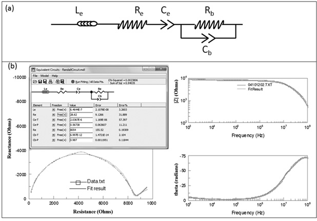
Fig. 2: ZView circuit and analysis of the data obtained from the impedance analyzer (a) Equivalent circuit diagram as used in the Z view software. With respect to the circuit shown in Fig 1: the two electrodes are lumped together, the bulk and interfacial capacitances have been replaced by Constant Phase Elements (CPEs), and the inductance of lead wires included (b) Results obtained using Z-view®, when the data from Impedance Analyzer (solid line with dots) was fitted to the circuit model (solid line without dots)
A CPE is a non-intuitive circuit element that replaces a capacitor in a circuit when the there is some type of non-homogeneity in the system, delaying or impeding the movement of charge carriers[27]. Mathematically, a CPE is an element whose impedance is given by the equation
Z = 0 – j (1/(wQ)n) …(4)
where Q is the magnitude and n is the phase angle of the CPE. It may be noted that when n equals 1, the impedance of the element is identical to that of an ideal capacitor with the same magnitude. Because ions need time to migrate from the bulk solution to form the “double layers”, electrode-solution interfaces are often modeled using CPEs28. Assuming that capacitances in the interior also require a finite time to be formed, we have chosen to replace the bulk capacitance with a CPE as well.
The software is written for use in Electrical / Electrochemical Impedance Spectroscopy. It accepts as input, the measured values of Resistance (R) and Reactance (X) at multiple frequencies, allows the user to propose an equivalent circuit for the material being investigated, and provides an estimate of the values of the individual elements in the equivalent circuit (Le, Re, Ce, Rb, CPE-T, and CPE-P in our case), along with an “error” of the estimate. If we are able to unequivocally establish that, after a certain duration of incubation, the value of the magnitude of the CPE (the CPE-T parameter) has increased (implying that the number of charge-storing species in the suspension’s interior has increased), it can be attributed to microbial proliferation (and hence presence of viable microorganisms) in the original sample.
By providing estimates of each individual parameter, the software allows the user to distinguish changes to the overall impedance occurring due to an increase in the Bulk Capacitance of the suspension on account of microbial proliferation (our phenomenon of interest) from changes in other factors (if any). For instance, small changes in temperature changes would be expected to change the conductivity of the solution significantly29, which would result in a change in the bulk resistance (Rb) while leaving the Bulk Capacitance (Cb), which arises from cell-membrane polarization, largely unaffected30. Also with time, the surface of the electrode may undergo corrosion as a result of which the properties of the electrode/electrochemical interface (Le, Re and Ce) may change31. The interfacial capacitance (Ce) may also change due to change in pH and temperature since the ions in the interfacial “double layer” are in electrochemical equilibrium with the bulk32. However, our analysis of the Z vs. ù data allows us to calculate changes to all parameters, individually. By focusing exclusively on the change in the Bulk Capacitance, we are able to proceed effectively, despite the occurrence of these other phenomena.
Times to detection (TTDs)
The ZViewTM software generates not only an estimate of the parameters (such as the Bulk Capacitance, CPE-T value), but also an “error”. For two recorded values to be “significantly” different from each other, there should not be any overlap between the ranges ([value – error] to [value + error]) of the two readings. As we calculate the value of the Bulk Capacitance after various intervals of time, we examine whether or not the present value is “significantly” greater than the initial (0-hour) value. A “significant” increase in the Bulk Capacitance value would indicate an increase in the number of species capable of storing charge that are dispersed in the medium. Since other such species (such as proteins and blood cells in the case of Blood Culture, milk proteins and fruit pulp in food substrates, silica particles in environmental samples, etc.) are not expected to increase in number, such an increase can only be brought about by microbial proliferation, as is hence taken as a signature of the presence of proliferating microorganisms in the sample. The time taken to obtain such a “significant” increase in the value of the Bulk Capacitance is our Time to Detection (TTD). The TTD is a function of the initial load, doubling time and the “threshold concentration”, and is given by the relation
TTD = 1.443 tD ln (nT/n0) … (5)
where
tD is the Doubling time of the microorganisms
n0 is the Initial Concentration, and
nT is the Threshold Concentration
Threshold concentration is defined to be the concentration of viable and proliferating microorganisms in the sample at the point in time that our method can unequivocally discern a change in the bulk capacitance from its baseline (t=0) value. It thus also depends on the magnitude of the baseline value (and hence the composition) of the suspension being assayed. A suspension with a higher baseline bulk capacitance will tend to have a higher threshold concentration. Consider two samples with baseline bulk capacitances of 2 and 10 pF, respectively. Assuming that our instrument/data analysis software can discern a 5% change in either, the proliferating microorganisms would have to contribute a capacitance of 0.1pF in the first case, and 0.5pF in the second to bring about these discernible changes. The latter sample would thus need to have more microorganisms generated in order for us detect the original proliferating members, and consequently, it will have a higher threshold concentration.
Quantifying the number of bacteria present [Most Probable Number (MPN)]
Although the value of the Bulk Capacitance (Cb) increases with an increase in the number of living bacterial cells present in a suspension, it is not possible to infer a bacterial count from reading the value of the Cb alone. This is because numerous other non-living species, such as proteins25 and inorganic nanoparticles13 (if present) will also contribute to the value of the Cb. The contributions from these non-living species will vary from one sample to another, but will not rise over time for a given sample. As a consequence, in order to quantify the number of living bacteria present, we have to rely on using the Most Probable Number (MPN)33-34 approach.
The MPN is a statistical method used to estimate the concentration of proliferating bacteria in a sample of interest that is widely used to monitor food and water quality. Briefly, and as depicted schematically in Figure 3, it involves serially diluting (by successive factors of 10) a known volume of the sample into bacterial growth media, culturing the “dilution series” bottles obtained for a sufficiently long period of time, and identifying the bottles that are “positive” (where growth of bacteria has occurred). If the sample originally had (say) 500 CFU/g, and we dissolved 1 g in 1ml of nutrient media to obtain our first solution (with 500 CFU/ml), the subsequent factor-of-ten dilutions should (under ideal conditions) contain 50, and 5 bacteria. A further factor-of-ten dilution will result in a solution with 1 CFU half the time, and 0 CFU on the other occasions (Probability of ½ that the sample contains one CFU). The probability that the next tenfold dilution will contain 1 CFU is 0.05 (5%). Further dilutions will have even lower probabilities of containing 1 CFU. If a given dilution series bottle contains even 1 CFU to begin with, it will ultimately (if cultured for a “sufficiently” long period of time) turn “positive” (display signs of bacterial presence like turbidity). By repeating the dilution experiments a number of times (typically 3 or 5), it is possible to obtain from the number of samples turning positive at each level of dilution, a statistical estimate of the number present in the original suspension. These estimates are available in literature as tables.
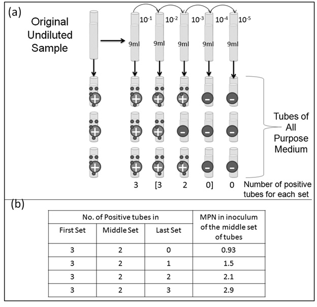
Fig. 3: The experimental protocol and statistical table for the most probable number (MPN) method (a): Schematic of most probable number (MPN) method briefly describing the protocol for the experiment (b) represents an extract from the statistical MPN determination table through which MPN and in turn the actual concentration of bacteria in the original sample can be determined
The key to obtaining correct MPNs is to run the culture for a sufficiently long time so that even 1CFU in the whole suspension (typically 10ml) is detected. Using current systems (that typically use turbidity measurements to detect the proliferation of bacteria), bacterial concentrations have to rise to ~ 107 CFU/ml (or higher)35 before they can be identified as positive. Our method, as mentioned earlier, identifies samples as “positive” when the calculated value of the Bulk Capacitance increases “significantly” from the baseline (t=0) value of the sample. Because this “significant” change occurs for filtered growth media when the concentration of bacteria reaches a threshold of ~103 CFU/ml, our method19 can potentially identify positive samples much earlier. Also samples that do not turn positive before a certain “cutoff time” are typically deemed negative. Since with our method, even one CFU (if present) would be detected much earlier, we can potentially use a cutoff time much shorter than the 24 hrs typically used currently [36]. We should hence be able to cut down the time needed to determine the MPN.
Microbial cultures
Pseudomonas aeruginosa (ATCC 9027) (fast growing aerobic bacteria), Methylobacterium mesophilicum (ATCC 29983) (slow growing aerobic bacteria), Propionibacterium acnes (isolate) (Anaerobic bacteria), Dekkera anomala (ATCC 10559) (Yeast), Aspergillus brasiliensis (ATCC 16404) (Mold) are used in the experiments. A brasiliensis spores were obtained from Microbiologics Inc. in the form of pellets known to contain ~103spores/pellet, and used directly. The other organisms were originally obtained in lyophilized form from ATCC, and log-cultures preserved in glycerol solution within cryotubes prior to use for the experiments described.
Sample preparation
The microorganisms in the cryotubes are taken from the freezer (-20oC) and thawed to reach room temperature. Immediately on thawing, 100µl of the solution in the cryotube is diluted into 900µl of 0.1% peptone water. These samples are then serially diluted in 0.1% peptone water (by appropriate factors, depending on the concentrations of the specific organisms present in the cryotubes) to yield solutions containing ~106 CFU/ml of the microorganism. 1ml of this 0.1% peptone water suspension containing ~106 CFU/ml of the microorganism is added to 9 ml of appropriate media (as listed in Table 1) to yield cultures with initial loads of ~105 CFU/ml. These cultures are incubated at desired temperature for different amounts of time to obtain “log cultures” with ~ 108 CFU/ml of microorganisms. In Table 1, we list the estimated CFU/ml of microorganisms in the cryotubes, the liquid media in which they are subsequently cultured, the temperature of culture, and the time for which they were cultured to obtain log cultures. These log cultures are then serially diluted in 0.1% peptone water and appropriate volume of the samples containing microorganisms are added to respective sterile media (listed in Table 1) to yield the “incubation study” media, which are then cultured at conditions mentioned in Table 1.
Table (1):
Experimental parameters used for testing microorganisms of interest.
M. mesophilicum ATCC 29983 |
P. aeruginosa ATCC 9027 |
P. acnes (isolate) |
D. anomala ATCC 10559 |
A. brasiliensis |
|
|---|---|---|---|---|---|
Expected CFU/ml in Cryotube |
4 x 10⁷ |
2 x 10⁸ |
8 x 10⁶ |
5 x 10⁶ |
– |
Broth in which cultured |
R2A |
Tryptic Soy Broth |
Fluid thioglycollate medium |
SAB |
SAB |
Incubation condition |
Standing |
standing |
Standing |
standing |
Standing |
Incubation temperature |
20 to 25ºC |
20 to 25°C |
30 to 35°C |
20 to 25ºC |
20 to 25ºC |
Time between Electrical measurements |
6 hrs |
1 hr |
2 hrs |
6 hrs |
6 hrs |
Agar used for plate counts |
R2A |
Tryptic Soy Agar |
Reinforced Columbia agar |
SDA |
SDA |
For A brasiliensis, the pellet (containing 103 CFU) is re-suspended in 0.1% peptone water to give 103 spores/ml of microbial concentration. 1 ml of this sample was added to 9 ml of Sabouraud Dextrose Broth (SAB), to give an estimated initial load of ~ 100 CFU/ml which was later confirmed by the plate counts on Sabouraud Dextrose Agar (SDA). This is directly used for impedance measurements without creating a log culture growth as for microorganism in cryotubes. Periodically, (every 1 to 6hrs, depending on expected doubling time of the microorganisms) aliquots from these different media are drawn and assayed electrically using our impedance measurements. Parallel aliquots are plated on appropriate nutrient agar, and colony counts obtained after incubation for suitable length of time.
MPN experiments
As in the manner described in section 3.2, log-cultures of E coli (K12) in TSB, with bacterial concentrations ~109 CFU/ml, are obtained. 1ml of this sample taken in an Eppendorf tube, centrifuged for 8 mins at 6000 rpm and the pellet (bacteria) is re-suspended in 1ml of sterile fresh PBS. This is serially diluted in 1ml of PBS to obtain 1ml of buffer with ~103 CFU/ml of E coli. This serves as our “original sample”, analogous to the “real world” scenario of a sample of water collected from a source of interest (typically ~10L) and concentrated 1000-fold (to ~10ml)37.
This 1ml of “original sample” is then added to 9ml of sterile TSB (in a sterile 15ml centrifuge tube) to obtain 102 CFU/ml of E. coli and then serially diluted to obtain 10 CFU/ml, 1 CFU/ml 0.1 CFU/ml, and <0.1CFU/ml. This serial dilution step is repeated to make 3 sets of these same dilutions. This is then incubated at 37oC in an incubator shaker (Mini 4450 Shaker, Thermo ScientificTM) and every 2 hours, ~250µl of sample is taken, injected in microfluidic cassette (treated in a manner similar to that described in section 3.2) and the sample is assayed electrically using our method (described in detail in section 3.4). The measurements are run for a total of 12 hours.
The traditional MPN protocol38 is also implemented on the same samples. The samples, from which aliquots are drawn for electrical assay by our method, are incubated for an additional 12 hours (after we have ceased taking our electrical readings) for observation of visible bacterial growth (change of turbidity), as is typically done in MPN experiments. The results obtained by the two methods are then compared.
Multi-frequency Impedance Measurement and Data Analysis
Our method involves drawing a 250µl aliquot at regular time intervals from our suspension of interest, and introducing the aliquot into a microfluidic cassette with electrodes at specified locations. The Electrical Impedance (Z) between the electrodes is measured at multiple frequencies (ù), and the Z vs. ù data is analyzed offline to determine the bulk capacitance (Cb) of the suspension.
The Impedance (Z) measurements are made using an Agilent 4294A Impedance Analyzer (Agilent technologies, CA, USA) at multiple frequencies (ù) from 1 kHz to 100 MHz. To obtain the Impedance at a given frequency, the Impedance Analyzer generates a 500mV (peak to peak) voltage at that frequency, and records the magnitude and phase of the AC current through the sample as a result of the application of the same. It also takes as inputs the frequency range to be scanned (1 kHz to 100 MHz in our case) and the number of points desired (500, the maximum possible, in our case) and selects logarithmically equi-spaced frequencies. It records the measured values of R and X corresponding to each frequency (ù) in an ASCII file. The data in this file are analyzed off-line using software ZViewTM.
Data obtained from the Impedance Analyzer is fit to the equivalent circuit shown in Figure 2, (displayed using the software ZViewTM). The software is written for use in Electrical/ Electrochemical Impedance Spectroscopy. It accepts as input measured values of Resistance (R) and Reactance (X) at multiple frequencies (or, equivalently, the magnitude of the Impedance (Z) and the phase angle (q)), allows the user to propose an equivalent circuit for the material being investigated, and provides an estimate of the values of the individual elements in the equivalent circuit (Le, Re, Ce, Rb, CPE-T, and CPE-P in our case), along with an “error” of the estimate. By providing estimates of each individual parameter, the software allows the user to distinguish changes to the overall impedance occurring due to an increase in the bulk capacitance, from other factors, such as changes to the bulk resistance (For instance, temperature swings can change to the electrical conductivity of the solution, which in turn changes the bulk resistance).
The number of viable microorganisms in a suspension affects the value of the Bulk Capacitance (Cb). If the number of microorganisms increase (due to proliferation) then the value of Cb increases. For any study where the objective is merely to ascertain whether or not there are any proliferating microorganisms in a sample of interest, a “significant” increase in the value of Cb from its value at t=0 implies that there is an increase in the numbers of those physical elements that contribute to the bulk capacitance. Hence a significant increase in Cb, if observed, serves to confirm the presence of viable (capable of proliferation) microorganisms in the original sample and when such an increase is observed, the sample is deemed Positive by our method. However, it may be noted that if there happen to be bacteria present that are alive and metabolizing, but not reproducing (such as “Viable but Not Culturable” cells) the method will not be able to detect them.
The use of this criterion is illustrated in Figure 4. As seen, initially (at t =0), the magnitude of the CPE (diamond) is 1.96 + 0.024 Pico-Farads. The range of values is represented by the error bars. The value of Bulk Capacitance after 6 hours of incubation (obtained based on Impedance measurements taken at that time) is 1.99 + 0.024 Pico-Farads. As seen, the range overlaps with that of the 0-hour value (shaded region). Thus while we know in retrospect (from the colony counts of aliquots drawn at the time the impedance measurements are taken) that the number of bacteria increased (from ~10 to ~20 CFU/ml of suspension), the increase did not cause a “significant” change in the value of the Bulk Capacitance. Similarly, for 12, and 18 hour reading, the bulk capacitance value does not change significantly compared to 0 hour. However, the magnitude of the CPE at the 24 hour mark (2.07 + 0.024 Pico-Farads) is “significantly” different from the 0-hour value (2.07 – 0.024 = 2.046 > 1.984 = 1.96+ 0.024). Thus 24 hours is our Time to Detection (TTD) for this sample (indicated by the solid arrow). The threshold concentration can be estimated from the plate count obtained from the sample plated at TTP. In the case shown in Figure 4, it is (as indicated by the dotted arrow) ~1000 CFU/ml.
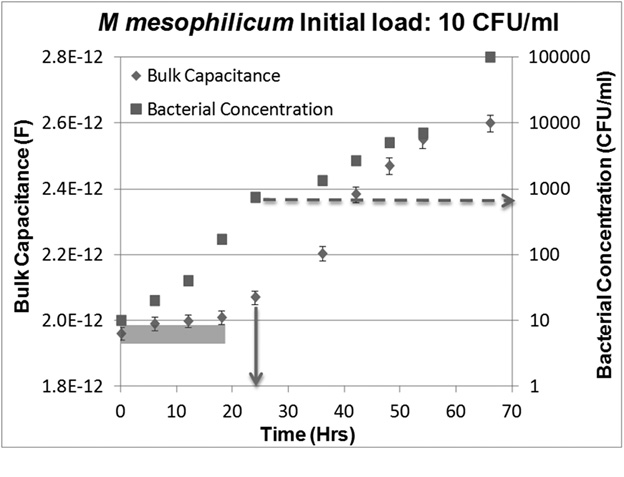
Fig. 4: Plot showing how the magnitude of the CPE of the bulk solution (Diamonds) and the concentration of microorganisms (Squares) evolve over time during culture in a sample with an initial load of ~10 CFU/ml of M mesophilicum. While microbial concentrations increase monotonically, magnitudes of CPE measured at 6, 12, and 18 hrs do not differ significantly from the 0-hr value (error bars overlap). A significant increase recorded only at 24 hrs, making this the Time to Detection (TTD) (solid arrow). The microbial concentration in the culture broth at TTD, the “threshold concentration”, for this sample is ~1000 CFU/ml, as shown by the dashed line
For determining MPN, the same principle is applied individually to all (diluted) samples to determine if there are any proliferating bacteria present, or not. Since our threshold concentrations are lower than that of current methods, we can detect the presence of bacteria much earlier, and also deem a sample to be negative in a correspondingly shorter time (8hrs, for the experiments conducted). The number of positives and negatives at each dilution, are recorded, and using statistical tables available in literature39, the MPNs estimated.
Rapid detection of proliferating microorganisms
In figure 5, we graphically present data from experiments conducted for all the microorganisms mentioned, with two different initial loads shown for each. Each graph shows the bulk capacitance values (diamonds) obtained by analyzing the electrical scans conducted at different points in time using the method described in section 3.4. The error-bars represent the standard error of the estimate, and are also provided by the impedance-analysis software (ZViewTM) used. Actual concentrations of the microorganisms in the culture broth at these times (found using plate culture, as described in section 3.2) are represented by squares. The times to detection for each sample (obtained using the criteria described in Section 3.4) are highlighted using solid arrow, and the threshold concentration (also obtained as described in Section 3.4) is highlighted using the dashed arrow. Table 2 gives the TTDs and the threshold concentrations for the different initial loads of the microorganisms tested.
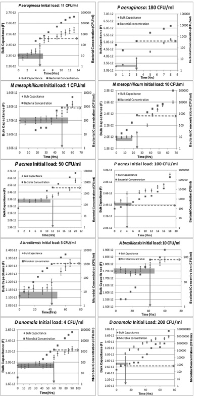
Fig. 5: Graphical representation of the results obtained using our method of detection for all the microorganisms, each with 2 different initial loads. Each graph represents the bulk capacitance values (Diamonds) and corresponding microbial concentrations (Squares) plotted over time. The solid arrow represents the TTD value for each microorganism at the given initial load, while the dashed arrow represents the threshold concentration at the time of detection
For the samples tested, the threshold concentration is of the order of 103 CFU/ml, irrespective of the identity of the organism. This threshold concentration is significantly lower than the threshold concentrations of current detection systems (107 – 108 CFU/ml)15. Also, as the concentration of viable cells rises by approximately 4 orders of magnitude (from ~10 to ~100,000 CFU/ml) the value of the Bulk Capacitance increases by approximately 40% (as can be seen in Figure 4). This is also a significant improvement over the performance metrics of existing technologies that perform the same function (determine the presence of actively proliferating microorganisms in suspensions). For instance, the BacT/Alert (a “gold standard” in Blood Culture i.e. for the detection of actively growing microbes in the blood) infers the presence of proliferating bacteria via a change in the level of CO2 in solution brought about by bacterial metabolism. The CO2 levels are measured via proprietary colorimetric molecules in the growth media. As described by Thorpe et al [8], a rise in the concentration of E coli from ~ 100 CFU/ml to ~ 107 CFU/ml (a rise in over 5 orders of magnitude) results in a change of ~15% in the “Reflectance Units” of the medium.
Our higher sensitivity, and more importantly, our lower threshold of detection, translates to faster times to detection, which in turn has important consequences in enabling clinicians/quality control scientists to make timely and effective decisions.
Dependence of TTD on initial load (n0) and doubling time (tD) of the micro-organism
In Table 2, it can be observed that Times to Detection (TTDs) are longer for lower initial loads for any given microorganism. Similarly, when comparing samples with similar initial loads (n0), microorganisms with a shorter doubling time (tD) such as Pseudomonas aeruginosa (for which tD = 1 hr 40) have a shorter TTD compared to microorganisms with a longer doubling time, such as Methylobacterium mesophilicum (for which tD = 8 hrs41). This is because, the microorganisms can be detected (caught in the act of increasing their numbers through reproduction) only when they have reached a certain threshold concentration. When we start with a low initial load, it takes longer to reach the threshold concentration and hence the samples have a longer TTD. Similarly, for similar initial loads, microorganisms with longer doubling-times need a longer amount of time to reach the threshold concentration. Hence there is a strong correlation between the doubling-times, initial loads of the microorganism and the TTDs.
Table (2):
TTDs for different initial loads of microorganisms and calculation of doubling times for various microorganisms.
Microorganism |
Initial Load (CFU/ml) |
Time to Detection (Hrs) |
Threshold Concentration (CFU/ml) |
Calculated Doubling time (Hrs) [90% Confidence Interval] |
Expected doubling time (Hrs) |
|---|---|---|---|---|---|
P aeruginosa |
11
180 230 |
5
5 2 |
390
2100 870 |
0.72
(0.04 – 1.39) |
0.75 – 1[40] |
M mesophilicum |
1
10 270 |
48
24 30 |
1000
750 4440 |
4.2
(-3.3 – 11.6) |
8 – 12[41] |
P acnes |
10
50 1000 |
16
12 4 |
2600
3500 1900 |
2.22
(2.07 – 2.35) |
1 – 2[43] |
A brasiliensis |
5
10 100 |
42
42 36 |
1000
400 1500 |
4.63
(3.66 – 5.59) |
6 |
D anomala |
4
60 200 |
60
42 12 |
1500
10000 800 |
7.88
(-2.8 – 18.57) |
6[44] |
If the surmise above is true, then mathematically, the Time to Detection (TTD) should be related to the initial load (n0) and doubling time (tD) of the microorganism by the equation
TTD = 1.443 tD ln (nT/n0) … (6)
In our experiments, the initial load in the sample and the threshold concentration can be estimated from the plate counts obtained at time t=0, and time t=TTD (as determined by analyzing the electrical data), respectively. By plotting the experimentally obtained values of TTD and nT for different samples (different n0 values) of the same organism, we should be able to estimate its doubling time (tD). If the estimated tD is found to be “reasonable”, this would indicate that our system behaves in the manner that is consistent with our understanding.
The above equation may be re-written as
TTD = 3.32 tD log10 (nT) – 3.32 tD log10 (n0) …(7)
Thus, if we plot TTD (y) of each sample against the log10 of initial loads (x), a regression analysis provides us with not just the values of the slope and intercept, but also the 90% Confidence intervals (CIs) of the same. Using the intercept values obtained from the regression line fit, and assuming an average threshold concentration of 1000 CFU/ml for all organisms, the doubling time (tD) for each microorganism along with 90% CI is calculated using equation 8
tD = Intercept /(3.32*log10(nT)) …(8)
We chose to use an “average” value of the threshold (rather than individual estimates for different experiments) because estimates obtained by standard plate counts itself is best regarded as an order-of-magnitude estimate42. The calculated values of doubling time (tD) in hours along with the 90% CI values (upper and lower limit values) are given in Table 2. The expected doubling time for each of these microorganisms are also given in the same table for comparison. It can be seen that the calculated doubling times (their 90% CIs) lie within the expected range for the doubling times for all microorganisms. Minor discrepancy in the values is expected as there is likely to have been an initial lag phase during microbial growth and also that the exact threshold concentration is likely to be slightly different for each microorganism.
Systems that are used to assay for the presence of living (metabolizing and reproducing) microorganisms in samples, such as BACTECTM and BacT/AlertTM used for blood culture, RABITTM and BactometerTM used for food and water quality measurement etc, are typically used to screen a large number of samples, and are required to yield “positive” results even for samples in which bacteria of different types are present (“mixed cultures”). Samples identified as “positive” are then analyzed using other techniques to identify the bacterial type(s) present (if identification is needed / desired). Our method, like the others mentioned above, also yields “positive” results for mixed cultures. On a few occasions, we have had contamination issues, when unknown bacteria were introduced into the sample. Such samples also yielded “positive” results (increase in bulk capacitance over time). However, because the initial load was unknown, the data could not be effectively analyzed to obtain relationships between initial load and Times to Detection. The evolution of Cb values over time, along with total colony counts (all types) for one such case has been has been provided in the supplemental material.
Determining the Most Probable Number (MPN) of proliferating bacteria
Each of the graphs shown in Figure 7 show how the Bulk Capacitance values of each of the 3 “tubes” at a given dilution of the “original sample” change with time. If a significant change in Bulk Capacitance is not observed within the duration for which measurements are taken (12 hours), then the particular tube is deemed negative. On the other hand, tubes are deemed positive as soon a significant change in Bulk Capacitance is recorded.
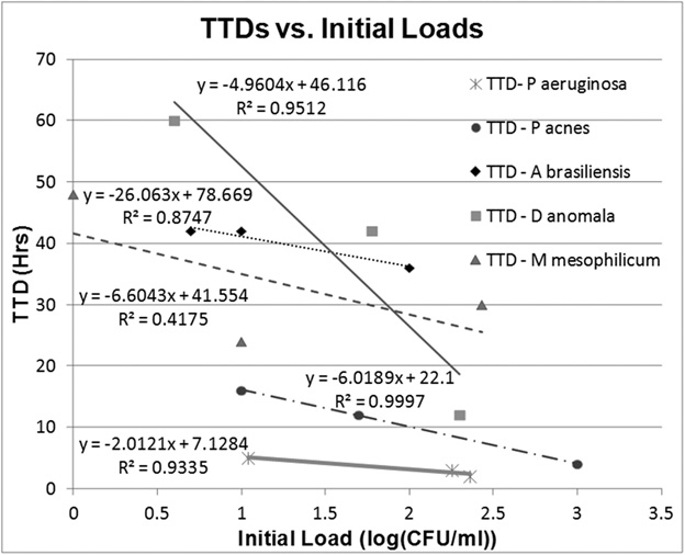
Fig. 6: Represents the plot of TTDs for all the sample microorganisms at different initial loads. The solid straight lines represent the regression lines of fit for each microorganism along with the equation of line
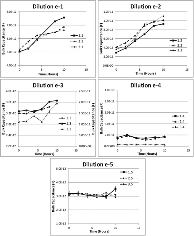
Fig. 7: Plots showing changes in the value of the measured Bulk Capacitance over time for samples containing different dilutions (e-1, e-2, e-3, e-4 and e-5) of the original sample (containing ~1000 CFU/ml) with the arrows indicating the TTD for the given dilution
From the plots shown in Figure 7 it can be seen that for all the tubes in the 1st three dilution series (which are expected to contain ~100, ~10 and ~1 CFU/ml), we can observe an increase in the value of the bulk capacitance (diamonds) over time indicating presence of bacteria in these tubes. This was also confirmed by presence of visible growth in the tubes after 24 hours of incubation. While for the 4th and the 5th dilution sets, with expected bacterial concentrations of ~0.1 CFU/ml (~ 1 CFU/10ml), and ~0.01 CFU/ml (< 1 CFU/100ml), there was no observed increase in the bulk capacitance values and also the TSB did not turn cloudy after 24 hrs of incubation (indicating the lack of bacteria).
The bacterial culture results (whether positive or negative) for all tubes are summarized in Table 3. For any given dilution, the number of tubes turning positive using traditional evaluation method (check for turbidity in the originally-clear medium after 24 hours of culture) is identified. This is compared (as shown in the table) to the result (positive or negative) obtained using our method. As seen, we obtained the “correct” result for all cases, and in all them, the positive samples were identified using our method in 2-6 hrs. (The solid lines in the graphs indicate the TTP for that particular tube).
Table (3):
Comparison of results obtained using our method and the traditional method for determining.
| Dilution Factor (Log10)0 | Tube Number | RESULTS | ||
|---|---|---|---|---|
| Traditional MPN (turbidity after 24 hrs of incubation) | Our method | |||
| Result | Time to Positivity (TTP) | |||
| -1 | 1 | Positive | Positive | 2 hours |
| 2 | Positive | Positive | 2 Hours | |
| 3 | Positive | Positive | 2 Hours | |
| -2 | 1 | Positive | Positive | 2 Hours |
| 2 | Positive | Positive | 2 Hours | |
| 3 | Positive | Positive | 2 Hours | |
| -3 | 1 | Positive | Positive | 6 Hours |
| 2 | Positive | Positive | 4 Hours | |
| 3 | Positive | Positive | 4 Hours | |
| -4 | 1 | Negative | Negative | — |
| 2 | Negative | Negative | — | |
| 3 | Negative | Negative | — | |
| -5 | 1 | Negative | Negative | — |
| 2 | Negative | Negative | — | |
| 3 | Negative | Negative | — | |
In order to estimate the concentration of bacteria in the original sample, we identified 3 sets of dilution tubes which shows the dilution of organisms “to extinction” –i.e., 3 successive sets of tubes where the indication for bacterial presence goes from positive to negative. For our experiment, it was [3, 0, and 0]. Now by using the 3 tube MPN table, and the obtained [3, 0, and 0] result, we can determine the MPN of bacteria in the samples to be 0.23 in the center tube (with a dilution factor of E-4 with respect to the original sample). Hence, the Most Probable Number (MPN) of organisms in the original undiluted sample to be is 2.3 X 10³ CFU/ml.
These results suggest that our method could be used to evaluate MPN significantly faster than traditional methods. In fact, the results suggest that a “cutoff time” of as low as 6 hrs can be used for coliforms (as opposed to 1-2 days, currently). This could have significant impact in a number of situations (such as those related to food quality and recreational water, as explained earlier).
In our previous work we had reported our ability to detect proliferating bacteria in food substrates [19] and blood cultures [20] in a significantly (4-10 fold) shorter amount of time, when compared to existing culture-based methods (automated culture systems). In this work, we have described in detail the protocols we use to acquire and analyze the data, and have explained the mathematical criteria that we use to identify samples in which proliferating microorganisms are present. More importantly, we have shown that the method is applicable to a wide variety of microorganisms (aerobic and anaerobic bacteria, fastidious bacteria, yeasts and molds), and all these microorganisms have similar detection thresholds, thereby making our method one suitable to a variety of applications. That the doubling times, calculated based on our hypothesized mathematical model for the behavior of the system and experimentally estimated threshold concentrations, are in line with expectations confirms that our understanding of how our system behaves is valid. In addition, we have presented “proof of principle” results showing how our basic method can also be adapted to determine the MPN of samples rapidly (again, 4-10 times more quickly than currently done).
As currently implemented, our system has one major drawback: viz. the need for periodic sampling. Manual sampling is not only tedious; it may also make the process economically non-viable. Moreover, there is always the chance of contamination being introduced when aliquots are drawn. We are hence currently in the process of developing an automated aseptic sampling system, that will not require manual intervention for the duration of the culture (hours to days). Once this system is developed, we plan on performing more experiments, especially with “unknown” or “field” samples, to establish the effectiveness of the method.
ACKNOWLEDGMENTS
The research was primarily funded using startup fund from the University of Missouri granted to SS. Part of the research project was also funded by EMD Millipore Corporation granted to SS. SP was supported in part by a Translational Research Award from the Coulter Foundation. BDL was also supported by funds from the Cheongbung scholarship foundation, South Korea.
- US Pharmacopeial Convention. In Book US Pharmacopeial Convention (Editor ed.^eds.). City; 2004.
- Teratanavat R, Hooker NH: Understanding the characteristics of US meat and poultry recalls: 1994-2002. Food control 2004, 15:359-367.
- Hayes MC, Boor K: Raw milk and fluid milk products. Applied dairy microbiology 2001:59-76.
- Doyle M: Microbial food spoilage–Losses and control strategies. In Book Microbial food spoilage–Losses and control strategies (Editor ed.^eds.). City: University of Wisconsin, Madison, WI; 2007.
- Anderson KA, Davidson PM: Drinking Water & Recreational Water Quality: Microbiological Criteria. University of Idaho, College of Agriculture, Cooperative Extension System, Agricultural Experiment Station; 1997.
- Dorfman MH, Stoner N, Rosselot KS, Council NRD: Testing the waters: a guide to water quality at vacation beaches. Natural Resources Defense Council; 2009.
- Horvath LL, George BJ, Murray CK, Harrison LS, Hospenthal DR: Direct comparison of the BACTEC 9240 and BacT/ALERT 3D automated blood culture systems for candida growth detection. Journal of clinical microbiology 2004, 42: 115-118.
- Thorpe TC, Wilson M, Turner J, DiGuiseppi J, Willert M, Mirrett S, Reller L: BacT/Alert: an automated colorimetric microbial detection system. Journal of clinical microbiology 1990, 28: 1608-1612.
- Woods GL, Fish G, Plaunt M, Murphy T: Clinical evaluation of difco ESP culture system II for growth and detection of mycobacteria. Journal of clinical microbiology 1997; 35: 121-124.
- Russell SM: Comparison of the traditional three-tube most probable number method with the Petrifilm, SimPlate, BioSys optical, and Bactometer conductance methods for enumerating Escherichia coli from chicken carcasses and ground beef. Journal of Food Protection 2000, 63: 1179-1183.
- Bolton F: An investigation of indirect conductimetry for detection of some food borne bacteria. Journal of Applied Microbiology 1990, 69: 655-661.
- Sengupta S, Gordon JE, Chang H-C: Microfluidic Diagnostic Systems for the Rapid Detection and Quantification of Pathogens. In. Edited by Finehout E; 2010
- Sengupta S, Battigelli D, Chang H: A micro-scale multi-frequency reactance measurement technique to detect bacterial growth at low bio-particle concentrations. Lab on a Chip 2006; 6: 682-692.
- Körner H, Zumft WG: Expression of denitrification enzymes in response to the dissolved oxygen level and respiratory substrate in continuous culture of Pseudomonas stutzeri. Applied and environmental microbiology 1989; 55: 1670-1676.
- Smith J, Serebrennikova Y, Huffman D, Leparc G, García Rubio L: A new method for the detection of microorganisms in blood cultures: Part I. Theoretical analysis and simulation of blood culture processes. The Canadian Journal of Chemical Engineering 2008; 86: 947-959.
- Noble RT, Weisberg SB: A review of technologies for rapid detection of bacteria in recreational waters. Journal of water and health 2005; 3: 381-392.
- Liu RH, Yang J, Lenigk R, Bonanno J, Grodzinski P: Self-contained, fully integrated biochip for sample preparation, polymerase chain reaction amplification, and DNA microarray detection. Analytical Chemistry 2004; 76: 1824-1831.
- Yang L, Bashir R: Electrical/electrochemical impedance for rapid detection of foodborne pathogenic bacteria. Biotechnology Advances 2008; 26: 135-150.
- Puttaswamy S, Sengupta S: Rapid detection of bacterial proliferation in food samples using microchannel impedance measurements at multiple frequencies. Sensing and Instrumentation for Food Quality and Safety 2010, 4:108-118.
- Puttaswamy S, Lee BD, Sengupta S: Novel Electrical Method for Early Detection of Viable Bacteria in Blood Cultures. Journal of clinical microbiology 2011; 49: 2286-2289.
- Asami K, Hanai T, Koizumi N: Dielectric analysis of Escherichia coli suspensions in the light of the theory of interfacial polarization. Biophysical Journal 1980; 31: 215-228.
- Shafiee H, Sano MB, Henslee EA, Caldwell JL, Davalos RV: Selective isolation of live/dead cells using contactless dielectrophoresis (cDEP). Lab on a Chip 2010; 10: 438-445.
- Pethig R, Markx GH: Applications of dielectrophoresis in biotechnology. Trends in biotechnology 1997; 15: 426-432.
- Rosen D: Dielectric measurements of proteins. In A Laboratory Manual of Analytical Methods of Protein Chemistry Including Polypeptides. Edited by Lundgren PAaH. New York: Pergamon Press; 1966.
- Sengupta S, Mahmud G, Chiou D, Ziaie B, Barocas V: Application of the lag-after-pulsed-separation (LAPS) flow meter to different protein solutions. The Analyst 2005; 130: 171-178.
- Chang HC, Yeo LY: Electrokinetically driven microfluidics and nanofluidics. Cambridge University Press; 2010.
- Barsoukov E, Macdonald JR: Impedance Spectroscopy: Theory, Experiment, and Applications 2nd edition edn: John Wiley & Sons, INc, New Jersey; 2005.
- Yao J, Gillis KD: Quantification of noise sources for amperometric measurement of quantal exocytosis using microelectrodes. Analyst 2012; 137: 2674 – 2681.
- Cussler EL: Heat Transfer. In Diffusion: Mass Transfer in Fluid Systems. Second edition: Cambridge University Press; 1997.
- Schwan HP, Foster KR: RF-field interactions with biological systems: electrical properties and biophysical mechanisms. Proceedings of the IEEE 1980; 68: 104-113.
- Baboian R: Corrosion Tests And Standards: Application And Interpretation. Second edn: ASTM international; 2005.
- Guyer J, Boettinger W, Warren J, McFadden G: Phase field modeling of electrochemistry I: Equilibrium. Arxiv preprint cond-mat/0308173 2003.
- Oblinger J, Koburger J: Understanding and teaching the most probable number technique. Journal of Milk and Food technology 1975; 38: 540-545.
- Sutton S: The Most probable Number (MPN) Method. Pharmaceutical Microbiology Forum Newsletter February, 2010; 16: 2 – 9.
- Lim DV: Growth and Control of Growth. In Microbiology. 3rd Edition edition: Kendall Hunt; 2002.
- Wrenn BA, Venosa AD: Selective enumeration of aromatic and aliphatic hydrocarbon degrading bacteria by a most-probable-number procedure. Canadian journal of microbiology 1996; 42: 252-258.
- Horan N: Handbook of water and wastewater microbiology. Academic Pr; 2003.
- Cochran WG: Estimation of bacterial densities by means of the” most probable number”. Biometrics 1950: 105-116.
- Salama IA, Koch GG, Tolley DH: On the estimation of the most probable number in a serial dilution experiment. Communications in Statistics-Theory and Methods 1978; 7: 1267-1281.
- Pearson JP, Passador L, Iglewski BH, Greenberg E: A second N-acylhomoserine lactone signal produced by Pseudomonas aeruginosa. Proceedings of the National Academy of Sciences 1995; 92: 1490.
- Sy A, Giraud E, Jourand P, Garcia N, Willems A, De Lajudie P, Prin Y, Neyra M, Gillis M, Boivin-Masson C: Methylotrophic MethylobacteriumBacteria Nodulate and Fix Nitrogen in Symbiosis with Legumes. Journal of Bacteriology 2001; 183: 214-220.
- Bhupathiraju VK, Hernandez M, Krauter P, Alvarez-Cohen L: A new direct microscopy based method for evaluating in-situ bioremediation. Journal of hazardous materials 1999; 67: 299-312.
- Hall GS, Pratt-Rippin K, Meisler DM, Washington JA, Roussel TJ, Miller D: Growth curve for Propionibacterium acnes. Current eye research 1994; 13: 465-466.
- Abbott D, Hynes S, Ingledew W: Growth rates of Dekkera/Brettanomyces yeasts hinder their ability to compete with Saccharomyces cerevisiae in batch corn mash fermentations. Applied microbiology and biotechnology 2005; 66: 641-647.
© The Author(s) 2017. Open Access. This article is distributed under the terms of the Creative Commons Attribution 4.0 International License which permits unrestricted use, sharing, distribution, and reproduction in any medium, provided you give appropriate credit to the original author(s) and the source, provide a link to the Creative Commons license, and indicate if changes were made.